Roster more effectively with Excel Ep1: Staffing level counts

Daniel Ge26 Sep, 20223 mins read

HOME→BLOGS→Roster more effectively with Excel Ep1: Staffing level counts

Have you ever wondered how to set up your rostering spreadsheet to quickly check if you have the right number of people on every day? Maybe you already have, but you would like some colour coding or even a quick check that every day is staffed correctly. In this post, I will go over some easy-to-implement excel formulas to do just that.

The setup

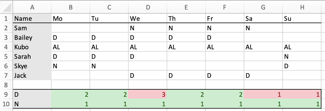
Let's imagine an oversimplified roster. Six people (though in this example, I've just chosen my friends' pets), and one week. Two shift types, "D" and "N". This pictured example has that as well as some leave (AL) and the counts we intend to achieve in place already.

Counting a shift

To put it simply, we want Excel to give us a count of all the D shifts on a given day. The COUNTIF formula will do this for us. COUNTIF counts all the instances of the text you're looking for within a range.

The basic version looks like this: =COUNTIF(B2:B57," D")

But it comes with a lot of extra work. Ideally, we want to write the formula once and be able to copy it while having it just work. For that, we'll need some relative references.

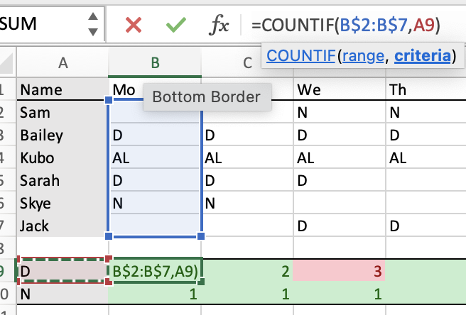
To do that, we use something like this: =COUNTIF(B2:B57,A9)

Now, instead of always looking for "D", when I copy my formula down a row, the formula will adjust and count the "N" s instead. However, I have introduced a pitfall for myself here.

The correct advanced version looks like this: =COUNTIF(B$2:B$57,A$9)

The '$' tells Excel that the part after '$' doesn't change when I copy this formula elsewhere. Without it, when I copied my formula down, it would have stopped counting Sam for the "N" shifts. The same thing applies when we move to the right, it would no longer be counting my "D" or "N" shifts.

Making Checking Easier

Once you've got those numbers in place, you might find as I did, that reading many numbers is a bit of a pain. I just want to see problem areas where there is something to address. To do this, let's add some coloured highlighting with conditional formatting to the range of numbers.

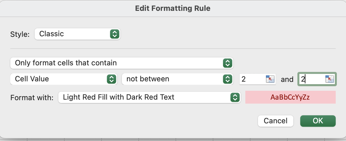
I have a formatting rule set up to warn me if I don't have 2 people on "D" for every day and 1 for every "N", as well as green to let me feel good that I got it right when I did. I'll just explain the process for the first warning. The process is the same, just with different configurations. Just select the range you want the highlighting to be on and then search for conditional formatting in the help bar.

Of course, this can get quite repetitive. We could set up a table of ideal numbers and use conditional formatting to check against those instead. Or you could try Rosterlab Free, which gives all this functionality and more out of all this hassle.

Skills Mix

We may also want to count how many people in each shift are in a given role. This is useful for ensuring that shifts are covered by a diverse mix of seniority levels. One common way of handling this is to cluster all the people of a role together, but this will lead to problems with your formulas when you try to add or remove people. With a COUNTIFS formula like in the image below, we can use the same formula and copy that across all our skill checks as well.

Hopefully, this has shown you how to up your rostering game within Excel. If these seem like good features you'd like to implement but are short on time or just don't want to put in the effort, try out Rosterlab Free. With Rosterlab Free, not only are all these features available but also features that help you check how fair your rosters are and if you're breaking any of your contractual, union, or workplace rostering guidelines.